The Transfer Function and Frequency Response¶

We use the notation of the overview: a filter with impulse response $h$, an angular frequency $\omega$, and the imaginary unit $i$. A filter is determined by its impulse response, but its action is often clearer in terms of the frequencies it passes and delays, which the transfer function encodes.

Definition: transfer function

The transfer function of a filter with impulse response $h$ is the Laplace transform $$ H(s) = \int_{0}^{\infty} h(t)\, e^{-st}\, dt $$ of $h$, a function of the complex variable $s$. It determines the filter completely.

The transfer function measures how the filter responds to the complex exponential $e^{st}$, which it reproduces scaled by $H(s)$. The physically meaningful exponentials are the pure oscillations $e^{i\omega t}$, obtained by restricting $s$ to the imaginary axis.

Definition: frequency response

The frequency response is the restriction of the transfer function to the imaginary axis, $s = i\omega$: $$ H(i\omega) = \int_{0}^{\infty} h(t)\, e^{-i\omega t}\, dt . $$ Written in polar form, $$ H(i\omega) = \lvert H(i\omega) \rvert\, e^{i\phi(\omega)}, \qquad \phi(\omega) = \arg H(i\omega), $$ its modulus $\lvert H(i\omega) \rvert$ is the magnitude response and its argument $\phi(\omega)$ is the phase response.

The magnitude response records the gain applied to each frequency, and the phase response records the corresponding shift. The two measures of delay treated in Phase Delay and Group Delay are both determined by $\phi$.

Example: a first-order low-pass filter

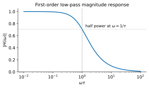
The filter with impulse response $h(t) = \tau^{-1} e^{-t/\tau}$ for $t \ge 0$ has transfer function $H(s) = (1 + s\tau)^{-1}$ and frequency response $$ H(i\omega) = \frac{1}{1 + i\omega\tau}, \qquad \lvert H(i\omega) \rvert = \frac{1}{\sqrt{1 + (\omega\tau)^2}} . $$ The gain is unity at $\omega = 0$, falls to $1/\sqrt{2}$ at the corner frequency $\omega = 1/\tau$, and decays as $1/(\omega\tau)$ beyond it: the filter passes slow variation and suppresses fast variation.

Magnitude response of a first-order low-pass filter, unity at DC and falling past the corner frequency

In discrete time

Sampling replaces the Laplace transform by the $z$-transform $H(z) = \sum_{n=0}^{N-1} h[n]\, z^{-n}$, and the imaginary axis by the unit circle: the frequency response is $H(e^{i\omega})$, the discrete-time Fourier transform of the taps. The magnitude and phase responses are its modulus and argument, as before.

Sampling the low-pass impulse response gives taps whose gain is unity at zero frequency, the sum of the taps, and which decay toward the Nyquist frequency:

import numpy as np
from scipy.signal import freqz

fs, tau = 2000.0, 0.05
n = np.arange(0, int(8 * tau * fs))
h = np.exp(-n / (tau * fs)) / (tau * fs)     # sampled low-pass impulse response
w, H = freqz(h, worN=1024, fs=fs)
assert np.isclose(np.abs(H[0]), 1.0, atol=1e-2)   # unit gain at zero frequency
assert np.abs(H[0]) > np.abs(H[-1])               # low-pass rolloff

References¶

Transfer function (Wikipedia).
Frequency response (Wikipedia).
Laplace transform (Wikipedia).
Z-transform (Wikipedia).